Energy of a Hydrogen atom

One of the most exciting aspects of quantum chemistry lies in solving the wavefunction of the hydrogen atom. Because it is the only system for which an exact analytical solution exists for both the energy levels and the atomic functions. For all other atoms, we must incorporate some approximations or tricky treatments in order to get fairly good results. The hydrogen’s wavefunction also provides the foundation for numerous concepts in quantum chemistry, including the concept of basis function, and the linearly combined molecular orbitals.

The Schrödinger equation for a Hydrogen atom

Hydrogen, the simplest element in the periodic table, consists of a single electron bound to a proton. In quantum mechanics, the energy and quantum state of a system are solutions of the so-called Schrödinger equation. For a hydrogen atom, the Schrödinger equation in atomic units is given by

\[\begin{equation} -\frac{1}{2}\nabla^2\psi-\frac{1}{r}\psi=E\psi \label{eq:schrodinger} \end{equation}\]

where $\nabla^2$ is the Laplace operator, which is defined in Cartesian coordinate as

\[\begin{equation} \nabla^2=\frac{\partial}{\partial x}+\frac{\partial}{\partial y}+\frac{\partial}{\partial z} \end{equation}\]

It is convenient to acknowledge the spherical symmetry of the problem by expressing the derivatives in terms of spherical polar coordinates. Standard manipulation of the differentials leads to the following expression for the laplacian operator

\[\begin{equation} \nabla^2=\frac{1}{r^2}\frac{\partial}{\partial r}\bigg(r^2\frac{\partial}{\partial r}\bigg)+\frac{1}{r^2\sin\theta}\frac{\partial}{\partial \theta}\bigg(\sin\theta\frac{\partial}{\partial\theta}\bigg)+\frac{1}{r^2\sin^2\theta}\frac{\partial^2}{\partial \phi^2} \end{equation}\]

This expression appears complex, where it involves three variables $r, \phi$, and $\theta$ represented in heterogenous patterns. However, we can see that the radial component $r$ does not mix with the angular components ($\phi,\theta$). This suggests that the Schrödinger equation for the hydrogen atom can be separable into angular and radial parts. Therefore, we propose a solution of the form

\[\begin{equation} \psi(r,\theta,\phi)=R(r)Y(\theta,\phi) \end{equation}\]

Substituting this into Equation \eqref{eq:schrodinger}, we obtain

\[\begin{equation} -\frac{1}{2}\bigg[\frac{Y}{r^2}\frac{\partial}{\partial r}\bigg(r^2\frac{\partial R}{\partial r}\bigg)+\frac{R}{r^2\sin\theta}\frac{\partial}{\partial\theta}\bigg(\sin\theta\frac{\partial Y}{\partial\theta}\bigg)+\frac{R}{r^2\sin^2\theta}\frac{\partial^2Y}{\partial\phi^2}\bigg]-\frac{1}{r}RY=ERY \end{equation}\]

Diving by $YR$ and multiplying by $-2r^2$, we get

\[\begin{equation} \bigg[\frac{1}{R}\frac{\partial}{\partial r}\bigg(r^2\frac{\partial R}{\partial r}\bigg)+2r+2Er^2\bigg]+\frac{1}{Y}\bigg[\frac{1}{\sin\theta}\frac{\partial}{\partial\theta}\bigg(\sin\theta\frac{\partial Y}{\partial\theta}\bigg)+\frac{1}{\sin^2\theta}\frac{\partial^2Y}{\partial\phi^2}\bigg]=0 \end{equation}\]

Obviously, the term in the first square bracket depends solely on $r$, whereas the remainder depends only on $\theta$ and $\phi$; accordingly, each must be a constant. Let say, they equal to $l(l+1)$, as we will see later that $l$ corresponds to the angular momentum quantum number.

\[\begin{equation} \frac{1}{R}\frac{\partial}{\partial r}\bigg(r^2\frac{\partial R}{\partial r}\bigg)+2r+2Er^2=l(l+1)\\ \frac{1}{Y}\bigg[\frac{1}{\sin\theta}\frac{\partial}{\partial\theta}\bigg(\sin\theta\frac{\partial Y}{\partial\theta}\bigg)+\frac{1}{\sin^2\theta}\frac{\partial^2Y}{\partial\phi^2}\bigg]=l(l+1) \end{equation}\]

In this article, we focus on the first equation, so-called radial equation. At this stage, we introduce a new variable $u=rR$, so that $R=u/r$, $\partial R/\partial r=[r(\partial u/\partial r)-r]/r^2$, and $(\partial/\partial r)[r^2(\partial R/\partial r)]=r\partial^2u/\partial r^2$, and hence

\[\begin{equation} -\frac{1}{2}\frac{\partial^2u}{\partial r^2}+\bigg[-\frac{1}{r}+\frac{l(l+1)}{2r^2}\bigg]u=Eu \label{eq:final_eqn} \end{equation}\]

The term inside the square bracket is called effective potential energy

\[\begin{equation} \tilde V=-\frac{1}{r}+\frac{l(l+1)}{2r^2} \end{equation}\]

and it has a physical meaning. The first part is the attractive Coulomb potential energy created by attractive force between electron and nucleus. The second part is a repulsive contribution that corresponds to the existence of a centrifugal force, which arises due to the nonsymmetric motion of the electron due to the angular momentum, and hence, applies for $l>0$. This force, on the other hand, impels the electron away from the nucleus. The competition between these two terms determines the electron’s behavior. At very short distances from the nucleus, the repulsive component tends more strongly to infinity (as $1/r^2$) than the attractive part (which varies as $1/r$), and the former dominates.

As you can notice, Equation \eqref{eq:final_eqn} is a second order differential equation for the function $u(r)$. Complete analytic solutions of this equation can be found in various ways, the book “Molecular Quantum Mechanics” by Peter Atkins and Ronald Friedman provides a straightforward section on using ladder operators, which is worth a look. Here, we will implement a numerical method in Python. The SciPy.integrate module is commonly used, particularly the odeint() function. The idea is to use odeint() to evaluate the first and second derivatives of the wavefunction $u$, which are subsequently used in the numerical integration. You can find the implementation somewhere in the internet (perhaps ChatGPT?). Instead, we will evaluate the second derivative of $u$ by using the finite difference approach. The Python implementation is adapted from this article.

The finite difference method is an approach to solve differential equations numerically. The approach approximates the derivative by the scheme

\[\begin{equation} \frac{du(r)}{dr}\approx\frac{u(r+h)-u(r)}{h} \end{equation}\]

In the finite difference scheme, the domain of the function is discretized with some finite step $h$. As a result, the convergence is quite sensitive to the magnitude of $h$. By the same manner, the second derivative is defined as

\[\begin{equation} \frac{d^2u(r)}{dr^2}\approx\frac{\frac{u(r+h)-u(r)}{h}-\frac{u(r)-u(r-h)}{h}}{h}=\frac{u(r+h)-2u(r)+u(r-h)}{h^2} \end{equation}\]

For the second derivative, we need to take into account at least three points of the discretized domain, which we chose $r-h,r,$ and $r+h$. Consider our problem

\[\begin{equation} -\frac{1}{2}\frac{\partial^2u}{\partial r^2}+\tilde Vu=Eu \end{equation}\]

We discretize the domain using a regular step of size $h$. The desired solution is the list of values $\psi(0),\psi(h),\psi(2h),\cdots,\psi((N+1)h)$, which we can index using an integer $i$. For each of these values, we can write down an equation of the form

\[\begin{equation} -\frac{1}{2}\frac{\partial^2u_1}{\partial r^2}+\tilde Vu_1=Eu_1 \end{equation}\]

where $N+2$ is the total number of points in the discretized domain. Using the approximation of the second derivative shown above, we have that

\[\begin{equation} \frac{-u_{i+1}+2u_i-u_{i-1}}{2h^2}+\tilde Vu_i=Eu_i\quad\forall i\in\{1,\cdots,N\} \end{equation}\]

This system of equations can be regarded as a single matrix equation

\[\begin{equation} \left[\begin{array}{cc} \frac{1}{h^2}+\tilde V & \frac{-1}{2h^2} \\ \frac{-1}{2h^2} & \frac{1}{h^2}+\tilde V &\frac{-1}{2h^2}\\ &\frac{-1}{2h^2}&\frac{1}{h^2}+\tilde V &\ddots\\ &&\ddots&\ddots&\frac{-1}{2h^2} \\ &&&\frac{-1}{2h^2}&\frac{1}{h^2}+\tilde V \end{array}\right]\left[\begin{array}{cc} u_1\\u_2\\u_3\\\vdots\\u_N \end{array}\right]=E\left[\begin{array}{cc} u_1\\u_2\\u_3\\\vdots\\u_N \end{array}\right] \label{eq:eigen} \end{equation}\]

which is in the form of an eigenvalue problem. Solving this, we find a set of eigenvectors $u$ representing the solution, and a corresponding set of eigenvalues $E$ which represent the energy levels.

It is pivotal to recognize the boundary conditions. The wavefunction must satisfy the Dirichlet boundary conditions $u_0=u_{N+1}=0$. This would imply two separate but trivial equations for the values $u_0$ and $u_{N+1}$. Moreover, as these values are zero by design, the differential operator is not affected by their presence. Hence, zero boundary conditions can be implemented by simply disregarding the equations for $u_0$ and $u_{N+1}$ completely, and only retaining the $N$ equations inside the discretized domain.

Python Implementation

We begin by generating the first matrix in Equation \eqref{eq:eigen} involving the discretized Laplace operator and the effective potential terms in a tridiagonal matrix. This matrix represents the Hamiltonian matrix to be diagonalized in order to solve the eigenproblem. Its eigenvalues are directly the energy states $E$, and the corresponding eigenvectors $u$ are related to radial part of the hydrogen wavefunction $R$ through the simple substitution we adopted earlier, $u=rR$. Remember the matrix takes in the variables: $r$ is the radial coordinate, and $l$ is the angular momentum number.

import numpy as np

def build_hamiltonian(r, l):
    h = r[1] - r[0]
    N = len(r)
    V_tilde = -1/r + l*(l+1)/(2*r**2)
    V_tilde = np.diag(V_tilde)
    main_diag = 1.0/h**2 * np.identity(N) + V_tilde
    off_diag = -1.0/(2*h**2) * (np.eye(N, k=1) + np.eye(N, k=-1))
    hamiltonian = main_diag + off_diag
    return hamiltonian

# Construct Hamiltonian matrix
N = 2000
l = 0
r = np.linspace(100, 0.0, N, endpoint=False)
hamiltonian = build_hamiltonian(r, l)

Now that we have the Hamiltonian matrix, we can proceed to solve the eigenproblem. Since the number of eigenvalues obtained through the diagonalization would be equal to the number of points $N$, there will be a number of positive eigenvalues. We are interested in the bound states with negative energies, and hence we limit ourselves to a couple dozen eigenstates with the smallest magnitude, in order to avoid the high energy solutions. Once computed, the eigenvalue and eigenvector pairs are to be sorted in ascending order.

# solve eigenproblem
eigenvalues, eigenvectors = np.linalg.eig(hamiltonian)

# sort eigenvalues and eigenvectors
eigenvectors = np.array([x for _, x in sorted(zip(eigenvalues, eigenvectors.T), key=lambda pair: pair[0])])
eigenvalues = np.sort(eigenvalues)

Since we chose $l=0$, we are sampling the hydrogen $s$ states ($1s,2s,3s,\cdots$). The exact energy for a hydrogen atom in eV is well-known as

\[\begin{equation} E_n=\frac{-13.6}{n^2}\quad n=1,2,\cdots \end{equation}\]

that agrees with our numerical solutions. You can tweak the value of $l$, but the same energies are obtained whatever the value of $l$, except for the removing some energy states. That’s because for any principal quantum number $n$, the permitted values of $l$ are $0,1,\cdots,n-1$. Hence, if for instance we choose $l=1$, the lowest energy solution is the one with $n=2$.

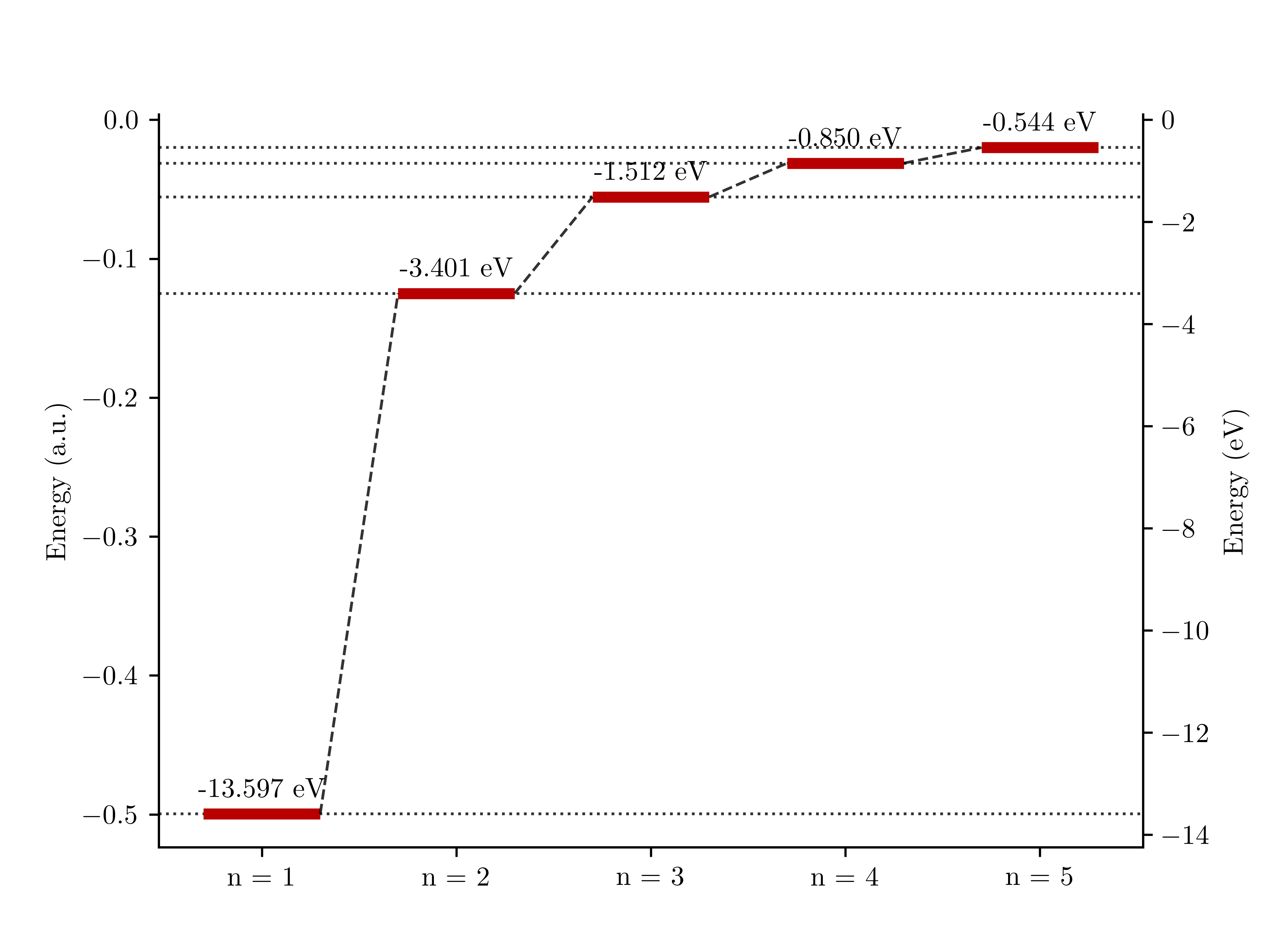
In principal, the energy in hydrogen atoms depends only on the principal quantum number $n$. Because $n$ are integers, the energy is also quantized. In addition, the higher values of $n$, the smaller gaps between two successive energy levels. You may also notice that not all the energy levels are found, especially for higher states. This is caused by the inadequacy of a regularly spaced grid in sampling the $1/r$ potential. Ideally either a coordinate transformation, or an adaptive grid would need to be used for a better sampling.

References

1. Introduction to Quantum Mechanics, 3rd Edition, Griffiths, D. J. & Schroeter, D. F.
2. Molecular Quantum Mechanics, 5th Edition, Peter W. Atkins, Ronald S. Friedman
3. The Problem of the Hydrogen Atom, Part 2, Physics, Python, and Programming