Orbitals of a Hydrogen atom

In the previous post, we numerically solved the Schrodinger equation for the hydrogen atom. Using a finite difference method implemented in Python, we are able to calculate the radial wavefunction and corresponding energy states. Our findings show that energy is not continuous but rather discretized. Additionally, the energy of hydrogenic atoms depends solely on the principal quantum number $n$. Today, we will focus on the properties of the total wavefunction, especially the angular part, for the hydrogen atom.

As indicated in the previous article, the complete wavefunctions of the electron in a hydrogenic atom have the form

\[\begin{equation} \psi_{nlm}(r,\theta,\phi)=R_{nl}(r)Y_{l}^m(\theta,\phi) \end{equation}\]

where $n,l,m$ indicate quantum numbers that determine a quantum particle’s state. For electrons in an atom, there are typically four quantum numbers:

• Principal quantum number ($n\geq1$) represents the electron’s energy level and relates to the radial distribution of the wavefunction. Quantum chemists normally consider the principal quantum number as the shell of an electron.
• Azimuthal quantum number ($0\leq l\leq n-1$), also known as orbital angular momentum quantum number, describes the subshell and relates to the shape of the atomic orbital. For example, $l=0$ indicates $s$ orbitals, $l=1$ are $p$ orbitals, $l=2$ are $d$ orbitals, $l=3$ are $f$ orbitals, etc.
• Magnetic quantum number ($-l\leq m\leq l$) specifies the orientation of the orbital in space. Because the values of $m$ range from $-l$ to $l$, the $s$ subshell ($l=0$) contains only one orbital, $p$ subshell ($l=1$) contains three orbitals, and so on.
• Spin quantum number ($m_s=1/2$ or $m_s=-1/2$) describes the electron’s intrinsic spin.

Note that the electron’s spin does not interact with anything else to affect its spatial distribution. Therefore, we will focus on the first three quantum numbers. A set of $nlm=1,0,0$ describes an electron in the $1s$ orbital, whereas $nlm=3,1,0$ describes an electron in the $3p_z$ orbital.

Radial wavefunction

The analytic formulas for the radial wavefunctions are related to the associated Laguerre functions

\[\begin{equation} R_{nl}=\sqrt{\left(\frac{2}{na_0}\right)^3\frac{(n-l-1)!}{2n(n+l)!}}e^{-\frac{r}{na_0}}\bigg(\frac{2r}{na_0}\bigg)^lL^{2l+1}_{n-l-1}\bigg(\frac{2r}{na_0}\bigg) \end{equation}\]

from scipy import special
import numpy as np

def radial_function(r, n, l):
    """ 
        n (int): principal quantum number
        l (int): azimuthal quantum number
        r (numpy.ndarray): radial coordinate
    """

    laguerre = special.genlaguerre(n-l-1, 2*l+1)
    
    # we will use the unit of Bohr radius
    a0 = 1
    rho = 2*np.abs(r)/(n*a0)

    constant_factor = np.sqrt(
        ((2/(n*a0))**3 * (special.factorial(n-l-1))) /
        (2*n * (special.factorial(n+l)))
    )
    return constant_factor * np.exp(-rho/2) * (rho**l) * laguerre(rho)

The physical interpretation for the radial wavefunction is its implication of probability of finding an electron in space. The probability that the electron will be found between $r$ and $r+dr$ is obtained from the radial distribution function

\[\begin{equation} P(r)=R_{nl}^2r^2 \end{equation}\]

def radial_distribution(r, n, l):
    return radial_function(r, n, l)**2 * r**2

You can notice that the probability density for each state is zero at $r=0$ (due to the factor $r^2$) and approaches zero as $r\rightarrow\infty$ on account of the exponential factor. There are two types of points that are of our interest. The first is where the probability of finding an electron is zero, which corresponds to a vanishing probability density. In chemistry language, this is referred to as a nodal point (or a node). Except for $r=0$, each radial wavefunction has $n-l-1$ nodes. The locations of these nodes are found by determining where the polynomial in the associated Laguerre function is equal to zero. The second type of point is where the electron is most likely to be found, which corresponds to the maximum value of the probability density. As seen in the $1s$ orbital, the probability density reaches a maximum at $r^{1s}_{\max}=a_0$, where $a_0$ is the Bohr radius. Therefore, the radius that Bohr calculated for the state of lowest energy in a hydrogen atom in his early pre-quantum mechanical model of the atom is in fact the most probable distance of the electron from the nucleus in the quantum mechanical model.

Angular wavefunction

The angular wavefunctions are spherical harmonics

\[Y^m_l=\sqrt{\frac{(2l+1)}{4\pi}\frac{(l-m)!}{(l+m)!}}e^{im\phi}P^m_l(\cos\theta)\]

where $P^m_l$ is the associated Legendre function.

def angular_function(theta, phi, m, l):
    """ 
        theta (numpy.ndarray): polar angle
        phi (numpy.ndarray): azimuthal angle
        m (int): magnetic quantum number
        l (int): azimuthal quantum number
    """

    legendre = special.lpmv(m, l, np.cos(theta))

    constant_factor = np.sqrt(
        (2*l + 1)/(4 * np.pi) *
        special.factorial(l - np.abs(m)) / special.factorial(l + np.abs(m))
    )

    y = constant_factor * legendre * np.exp(1.j * m * phi)
    
    # Linear combination of Y_l,m and Y_l,-m to create the real form.
    if m < 0:
        y = np.sqrt(2) * (-1)**m * y.imag
    elif m > 0:
        y = np.sqrt(2) * (-1)**m * y.real
    else:
        y = y.real
        
    return y

The angular wavefunction tells you the dependence of the wavefunction in terms of the polar ($\theta$) and azimuthal ($\phi$) angles. These spherical harmonics provide a detailed account of the shapes and orientations of hydrogenic orbitals, characterizing how electron probability distributions are spread out in space.

# Define quantum numbers
l, m = 2, 0
    
# Create matrices of polar, azimuthal angle points to plot
theta = np.linspace(0, np.pi, 100)
phi = np.linspace(0, 2*np.pi, 100)
theta, phi = np.meshgrid(theta, phi)

Yml = angular_function(theta, phi, m, l)

# Compute Cartesian coordinates of the surface
x = np.abs(Yml) * np.sin(theta) * np.cos(phi)
y = np.abs(Yml) * np.sin(theta) * np.sin(phi)
z = np.abs(Yml) * np.cos(theta)

# plot 3d surface
fig = plt.figure()
ax = fig.add_subplot(projection='3d')
ax.plot_surface(
    x, y, z,  
    cmap = "inferno_r",
)
ax.set_xlabel('X')
ax.set_ylabel('Y')
ax.set_zlabel('Z')
# make the panes transparent
ax.xaxis.set_pane_color((1.0, 1.0, 1.0, 0.0))
ax.yaxis.set_pane_color((1.0, 1.0, 1.0, 0.0))
ax.zaxis.set_pane_color((1.0, 1.0, 1.0, 0.0))
# make the grid lines transparent
ax.xaxis._axinfo["grid"]['color'] =  (1,1,1,0)
ax.yaxis._axinfo["grid"]['color'] =  (1,1,1,0)
ax.zaxis._axinfo["grid"]['color'] =  (1,1,1,0)
# make the ticks invisible
ax.set_xticks([])
ax.set_yticks([])
ax.set_zticks([])
ax.set_aspect("equal")
ax.set_title(f"l = {l}, m = {m}")

The angular wavefunction for the $1s$ orbital is constant for any values of $\theta$ and $\phi$. In this case, the angular dependence drops out and the wavefunction is spherically symmetric. This feature stems from its lack of orbital angular momentum. When $l\neq0$, the hydrogen angular wavefunctions are not spherically symmetric; they depend on $\theta$ and $\phi$, leading to unique orientation of the wavefunctions.

Total wavefunction

The radial part considers the distance from the nucleus, whereas the angular part characterize the spatial distribution. Together, they define the total wavefunction describing the electron’s behavior in the atom’s vicinity. Visualizing the hydrogenic wavefunctions is not easy. Chemists like to draw contour density plots, in which the color mapping of the cloud is proportional to $\psi^2$ which represents the probability density of the electrons’ presence in different regions of the atom. We can generate such a plot by taking a slice of $\psi^2$. Here we will plot the density in $xz$ plane, where the azimuthal angle $\phi=0$.

import matplotlib.pyplot as plt

# define quantum numbers
n, l, m = 3,2,0

# construct grid points
radial_extent = 50 # increase for high states
resolution = 100 # smooth the grid
x = z = np.linspace(-radial_extent, radial_extent, resolution)
y = 0 # xz plane
x, z = np.meshgrid(x, z)
# transform from Cartesian to spherical coordinate
r = np.sqrt((x**2 + y**2 + z**2))
eps = np.finfo(float).eps # Use epsilon to avoid division by zero during angle calculations
theta = np.arccos(z / (r + eps))
phi = np.arctan(y / (x + eps))

# Ψnlm(r,θ,φ) = Rnl(r).Ylm(θ,φ)
psi = radial_function(r, n, l) * angular_function(theta, phi, m, l)

# probability density
psi2 = psi ** 2

fig = plt.figure()
ax = fig.add_subplot()
# Find contours and plot
c = ax.contourf(psi2, cmap="magma")
cbar = fig.colorbar(c)
ax.set_xticks([])
ax.set_yticks([])
ax.set_title(f"n = {n}, l = {l}, m = {m}")

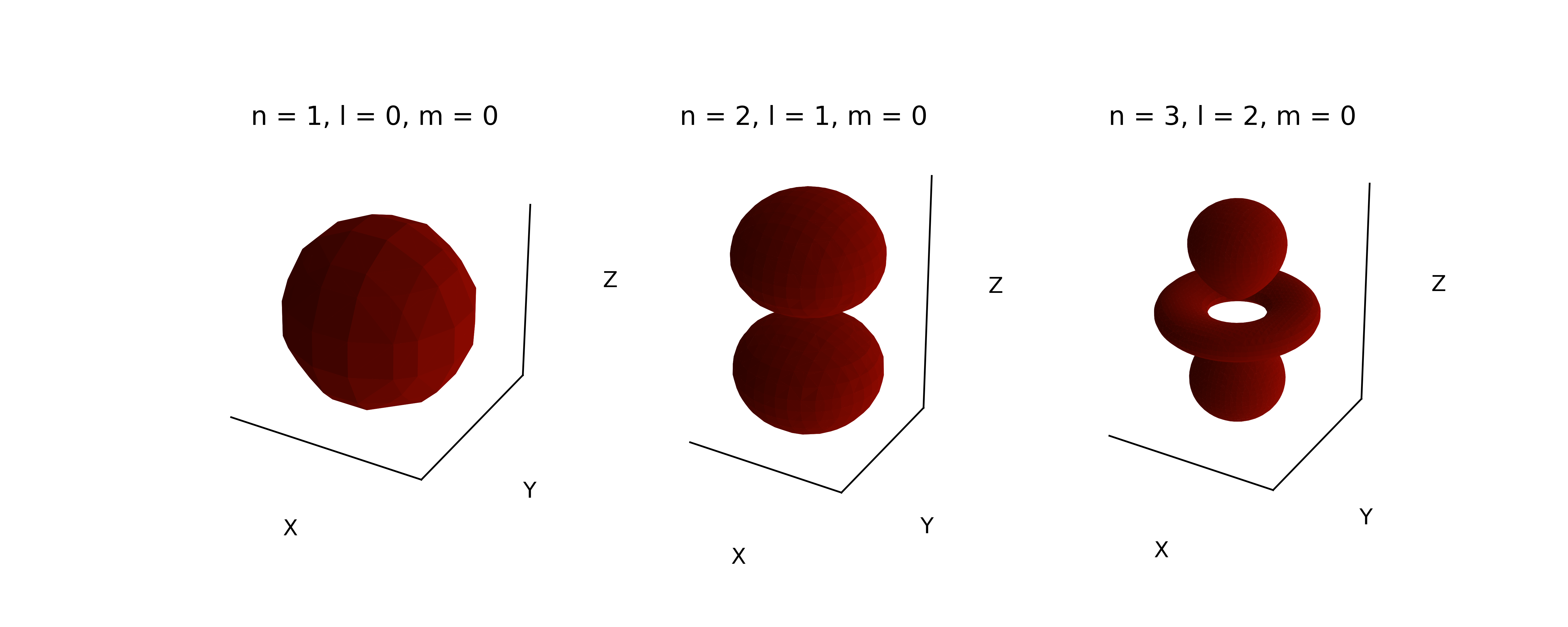
Alternatively, orbitals can be visualized in surfaces, similar to how we did for the angular wavefunctions. Recall that the square of the orbital at a particular point in space represents a probability density. As such, we can map values of the square of each orbital on a grid in 3-dimensional space, and then pick a threshold of probability density, and plot that as a contour surface. That surface is called an “isodensity” surface. To generate an isosurface from the probability density, we need to identify a grid of points where the density equals to a specific constant. A common algorithm for extracting isosurfaces from volumetric data is marching cubes, where cubic objects are iteratively checked if the surface pass through. In Python, the algorithm is implemented in skimage.measure.marching_cubes() function. For those who have not installed skimage package, please refer to the instruction.

import matplotlib.pyplot as plt
from mpl_toolkits.mplot3d.art3d import Poly3DCollection
from skimage.measure import marching_cubes

# define quantum numbers
n, l, m = 3,2,0

# construct grid points
radial_extent = 30 # increase for high states
resolution = 100 # smooth the grid
x = y = z = np.linspace(-radial_extent, radial_extent, resolution)
x, y, z = np.meshgrid(x, y, z)

# transform from Cartesian to spherical coordinate
r = np.sqrt((x**2 + y**2 + z**2))
eps = np.finfo(float).eps # Use epsilon to avoid division by zero during angle calculations
theta = np.arccos(z / (r + eps))
phi = np.arctan(y / (x + eps))

# Ψnlm(r,θ,φ) = Rnl(r).Ylm(θ,φ)
psi = radial_function(r, n, l) * angular_function(theta, phi, m, l)

# probability density
psi2 = psi ** 2

# define threshold within (0.0, 1.0) to construct isodensity surface
threshold = 0.15
level = (np.max(psi2)-np.min(psi2))*threshold + np.min(psi2)
verts, faces, normals, values = marching_cubes(psi2, level=level)

# Display resulting triangular mesh using Matplotlib
fig = plt.figure()
ax = fig.add_subplot(projection='3d')

# Fancy indexing: `verts[faces]` to generate a collection of triangles
mesh = Poly3DCollection(verts[faces], facecolors='#990a00', shade=True)
ax.add_collection3d(mesh)
ax.set_aspect('equal')
ax.set_xlabel('X')
ax.set_ylabel('Y')
ax.set_zlabel('Z')
# make the panes transparent
ax.xaxis.set_pane_color((1.0, 1.0, 1.0, 0.0))
ax.yaxis.set_pane_color((1.0, 1.0, 1.0, 0.0))
ax.zaxis.set_pane_color((1.0, 1.0, 1.0, 0.0))
# make the grid lines transparent
ax.xaxis._axinfo["grid"]['color'] =  (1,1,1,0)
ax.yaxis._axinfo["grid"]['color'] =  (1,1,1,0)
ax.zaxis._axinfo["grid"]['color'] =  (1,1,1,0)
# make the ticks invisible
ax.set_xticks([])
ax.set_yticks([])
ax.set_zticks([])
ax.set_aspect("equal")
ax.set_title(f"n = {n}, l = {l}, m = {m}")

References

1. Introduction to Quantum Mechanics, 3rd Edition, Griffiths, D. J. & Schroeter, D. F.
2. Molecular Quantum Mechanics, 5th Edition, Peter W. Atkins, Ronald S. Friedman
3. Quantum Mechanics with Python: Hydrogen Wavefunctions and Electron Density Plots